Loading...
Explore why Polars outperforms Pandas for file-based ETL above 1 GB. Understand the structural differences between eager single-threaded execution and Polars lazy multi-core evaluation, study benchmark evidence from real production migrations (94x on PDS-H, 17.5x at DB Systel), and apply a practical decision framework — including a hybrid approach for ML pipelines.
The tool that made Python data engineering accessible is quietly becoming the thing that slows it down.
Most Python data engineers learned pandas first. I was one of them as well. It was the standard, it worked, and it kept working well enough that nobody questioned it. That is exactly the problem.
Pandas was designed in 2008 for a different kind of data problem. It assumes you want immediate results from every operation, that a single CPU core is enough, and that data fits comfortably in RAM. Those assumptions held for years. They hold less and less as pipelines grow.
The question is not whether pandas is good. I know it is. I used it for years and it served me well. The question is if it still matches the shape of the workloads you are actually running.
For file-based ETL above roughly 1 GB, the answer is increasingly no. Not because pandas is broken, but because the ecosystem has produced something structurally better for that specific job. That tool is Polars. And the gap between the two is not marginal.
Before any benchmark numbers, the mechanism matters. I spent a long time treating Polars as "pandas but faster" before I understood why it is actually different. Once I did, the decision about when to use it became obvious. Understanding why it is faster tells you exactly when the advantage applies and when it does not.
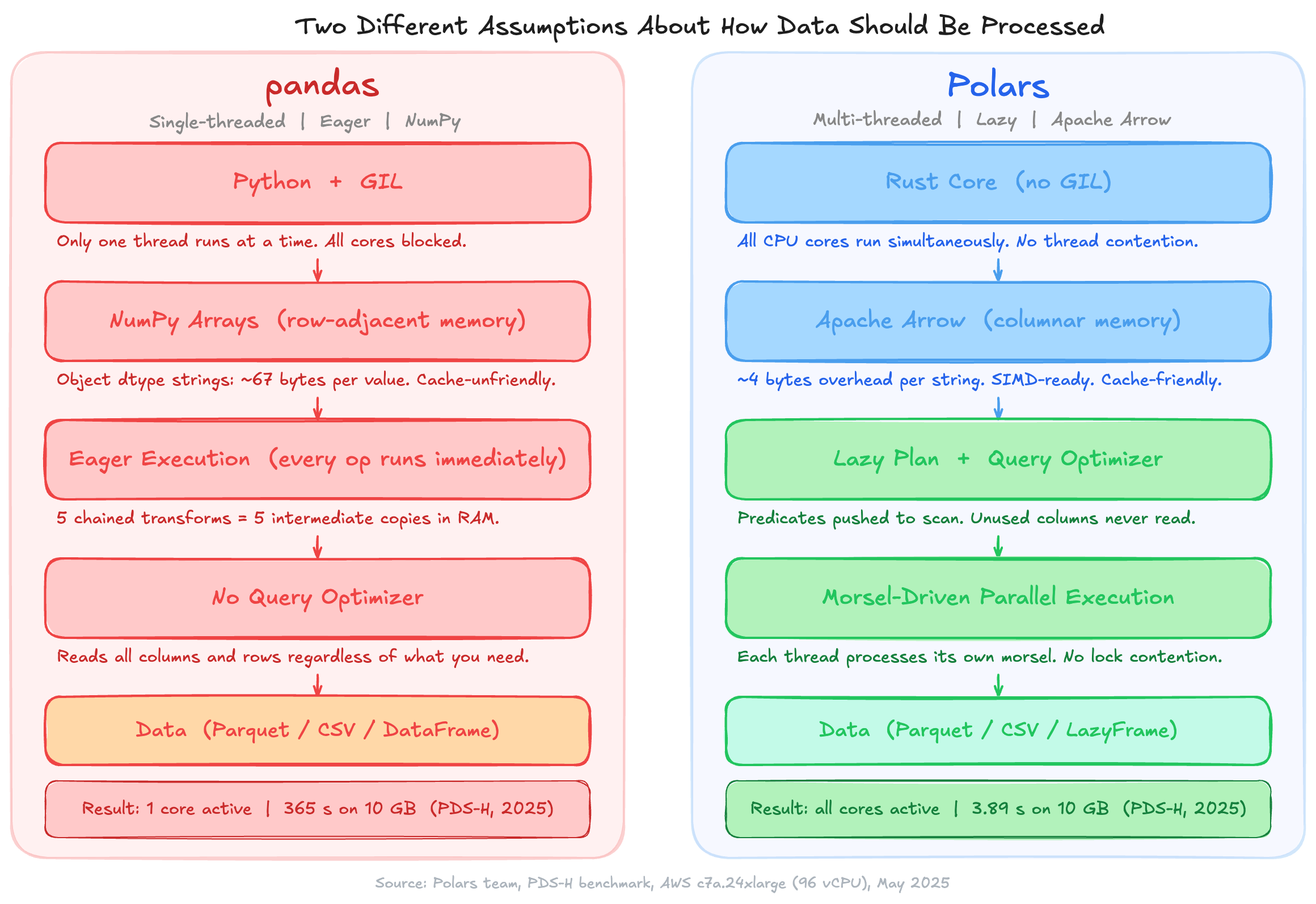
Pandas runs on NumPy, which is single-threaded for most operations. Python's Global Interpreter Lock prevents parallel execution even when multiple threads are available. Every operation runs immediately, which means intermediate results are created and stored in memory whether you need them or not. A chain of five transformations on a 5 GB DataFrame creates five intermediate copies. Memory usage compounds fast.
String columns make this worse. By default, pandas stores strings as NumPy object arrays: each value is a Python object pointer, consuming roughly 67 bytes per unique string versus 4 bytes of overhead in columnar storage. I first noticed this when a pipeline that should have used 3 GB of RAM was consistently consuming 9 GB. The culprit was a single string column on a wide DataFrame. A column of 1 million 18-character strings uses around 75 MB in pandas object dtype. The same column in Arrow format uses around 22 MB.
Polars is written in Rust and runs outside the GIL entirely. It stores data in Apache Arrow columnar format: each column is a contiguous block of typed memory, cache-friendly and SIMD-ready. When you call scan_parquet, no data is read yet. Polars builds a logical execution plan and optimizes it before touching a single byte: predicates are pushed down to the scan level, unused columns are pruned before reading, and joins are reordered for efficiency.
Execution is morsel-driven. Each CPU thread takes a chunk of input, processes it independently with its own local state, and merges results at the end. There is no lock contention during computation. All cores run simultaneously.
The practical consequence is something I measured myself, and the difference is not subtle. A pipeline that touches a 10 GB Parquet file in pandas reads all 10 GB, processes it sequentially on one core, and creates intermediate copies along the way. The same pipeline in Polars reads only the columns and row groups it needs, processes them in parallel across all cores, and never materializes an intermediate result it does not have to.
Three named tests establish the range of the gap.
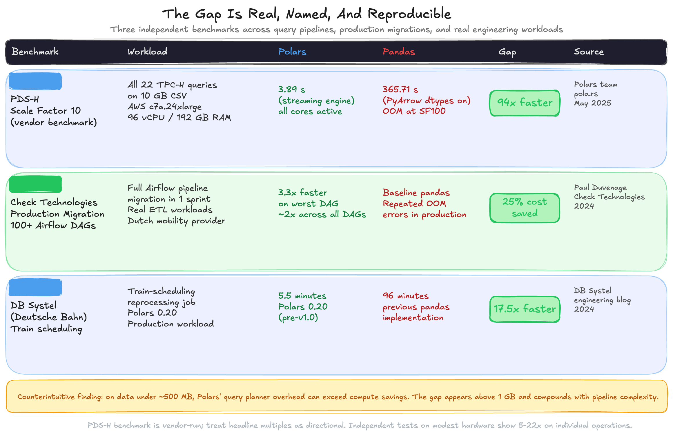
The Polars team published updated PDS-H results in May 2025, run on an AWS c7a.24xlarge instance with 96 vCPUs and 192 GB of RAM. The benchmark runs all 22 TPC-H-derived queries against a 10 GB CSV dataset. Polars streaming finished in 3.89 seconds. Pandas 2.2.3 with PyArrow dtypes enabled finished in 365.71 seconds. That is a 94x gap on a full multi-step analytical pipeline.
At scale factor 100 (100 GB), pandas was excluded entirely. Its single-threaded execution and lack of a query optimizer caused out-of-memory failures before completing the benchmark. Polars streaming finished in 23.94 seconds.
This is a vendor-run benchmark and I want to be clear about that. Treat it as directional, not as a universal promise. Independent tests on modest hardware consistently show smaller gaps, typically 5 to 22x on individual operations. The headline multiple emerges when the query optimizer and multi-threading compound across a full pipeline.
Check Technologies, a Dutch mobility provider, migrated all 100+ Airflow DAGs from pandas to Polars over a single sprint. Their motivation was not performance benchmarks — it was repeated out-of-memory errors on their most data-intensive pipelines. The migration took under two weeks and delivered a 3.3x speed improvement on the most problematic DAG, roughly 2x gains across almost all others, and a 25 percent reduction in cloud infrastructure cost.
DB Systel, a Deutsche Bahn subsidiary, rewrote a train-scheduling reprocessing job in Polars 0.20. The job previously ran in 96 minutes. The Polars version ran in 5.5 minutes. That is a 17.5x improvement on a real production workload, not a synthetic benchmark.
The counterintuitive finding: on small data, the gap largely disappears and sometimes reverses. Polars' query optimizer adds planning overhead that exceeds the compute savings when the dataset is under a few hundred megabytes. For quick scripts on small frames, pandas is faster to write and fast enough to run.
The setup is one command.
# Create project and add Polars
uv init polars-pipeline
cd polars-pipeline
uv add polars pyarrow  # standard install
uv run pipeline.py
No compilation. No system dependencies. Polars ships as a pre-built wheel with the Rust runtime included.
One thing worth knowing before you start: on Apple Silicon (M-series Macs), the standard polars wheel triggers a CPU compatibility warning and recommends the runtime-compatible variant.
# Apple Silicon: use this instead
uv add "polars[rtcompat]" pyarrow
On Linux and Intel Macs the standard install is fine. On M-series hardware, polars[rtcompat] avoids the warning and ensures the correct SIMD instructions are used for your processor.
When I first looked at Polars code, the syntax felt unfamiliar. The expression API takes a day to get used to. After that day, I found it more readable than the pandas equivalent, not less. The code below runs an identical ETL transformation: read a Parquet file, filter rows, aggregate by category, and sort the result.
# pandas version
import pandas as pd
import time

start = time.perf_counter()
df = pd.read_parquet("sales.parquet")
result = (
    df[df["revenue"] > 1000]
    .groupby("category")
    .agg(
        total_revenue=("revenue", "sum"),
        avg_price=("price", "mean"),
        order_count=("order_id", "count"),
    )
    .sort_values("total_revenue", ascending=False)
    .reset_index()
)
print(f"pandas: {time.perf_counter() - start:.3f}s")
print(result)
# Polars version — lazy execution with predicate and projection pushdown
import polars as pl
import time

start = time.perf_counter()
result = (
    pl.scan_parquet("sales.parquet")    # no data read yet
    .filter(pl.col("revenue") > 1000)   # pushed into the scan
    .group_by("category")
    .agg(
        total_revenue=pl.col("revenue").sum(),
        avg_price=pl.col("price").mean(),
        order_count=pl.col("order_id").count(),
    )
    .sort("total_revenue", descending=True)
    .collect()  # execution happens here
)
print(f"Polars: {time.perf_counter() - start:.3f}s")
print(result)
The structural difference is in scan_parquet versus read_parquet. The pandas version reads the entire file immediately. The Polars version builds a plan and reads only the rows and columns required to satisfy the filter and aggregation. On a 1 GB file with 20 columns where you need 3, Polars may read less than 20 percent of the bytes pandas reads.
When your dataset exceeds available RAM, add engine="streaming" to collect. Polars processes the data in batches called morsels, spilling to disk adaptively and never holding the full dataset in memory at once.
result = (
    pl.scan_parquet("large_dataset/*.parquet")
    .filter(pl.col("status") == "active")
    .group_by("region")
    .agg(pl.col("amount").sum())
    .sort("amount", descending=True)
    .collect(engine="streaming")  # out-of-core execution
)
For writing directly to disk without materializing in memory at all, use sink_parquet:
(
    pl.scan_parquet("raw/*.parquet")
    .filter(pl.col("error_code").is_null())
    .sink_parquet("clean/output.parquet")  # streams to disk in batches
)
Set thread count explicitly in production environments to avoid contention with other processes:
import os
os.environ["POLARS_MAX_THREADS"] = "8"  # MUST be set before importing polars
import polars as pl  # Polars initializes its thread pool at import time
Pin your Polars version in pyproject.toml. The API is stable at 1.x but minor versions introduce new features that change behavior on edge cases. Lock it, test in a container matching your production OS, and upgrade deliberately.
Polars is the better tool for file-based ETL on data above 1 GB. I still use pandas every week. There are three situations where I reach for it without hesitation.
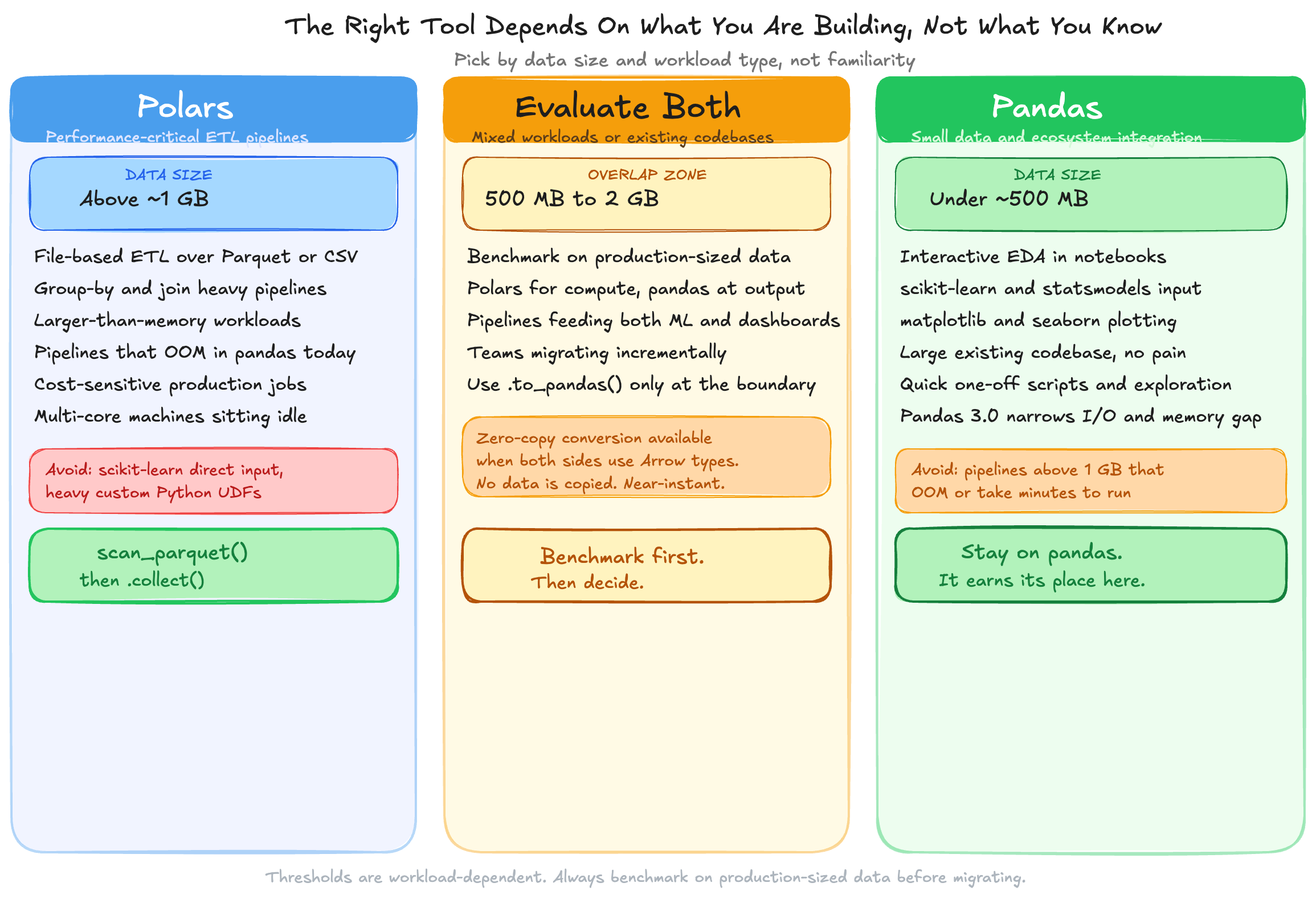
Most ML libraries accept pandas DataFrames as their native input format. scikit-learn, statsmodels, and many plotting libraries expect pandas either explicitly or by default. Rewriting your entire stack to avoid a single .to_pandas() call is not a trade-off worth making.
The practical pattern I use in every pipeline that feeds a model is the hybrid approach: Polars for the expensive compute work, then convert at the final step.
# Polars for the heavy lifting
features = (
    pl.scan_parquet("events/*.parquet")
    .group_by("user_id")
    .agg([
        pl.col("session_duration").mean().alias("avg_session"),
        pl.col("purchase").sum().alias("total_purchases"),
        pl.col("event_date").max().alias("last_seen"),
    ])
    .collect(engine="streaming")
)

# Zero-copy conversion at the boundary
X = features.to_pandas()  # Arrow-backed, near-instant
The conversion is near-instant because both Polars and recent pandas share the Apache Arrow memory format. No data is copied when both sides use Arrow types.
Pandas 3.0, released January 2026, made PyArrow-backed strings the default for string columns and made Copy-on-Write the only execution mode. These changes reduce memory usage on string-heavy datasets by up to 70 percent and eliminate a class of silent mutation bugs.
These are real improvements. They close the I/O and memory gap meaningfully. But they do not close the multi-core execution gap. Pandas aggregations remain single-threaded and eager with no query optimizer in any version. If your bottleneck is compute rather than memory, the 3.0 update does not change the calculus.
Three signals mean a pipeline is ready to migrate:
Any one of those signals is enough. All three together mean the migration pays back in the first sprint.
The starting point is narrow and concrete. Pick one pipeline — the slowest or the one that OOMs most often. Rewrite only the compute-heavy portion in Polars LazyFrame, keep the pandas boundary at the output for anything feeding into ML or plotting, and benchmark on production-sized data before promoting. If you do not see at least a 3x improvement on a dataset above 1 GB, the bottleneck is probably not the DataFrame library.